| Quantum Mechanics for Engineers |
|
© Leon van Dommelen |
|
D.83 Expectation powers of r for hydrogen
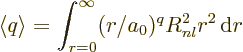
This note derives the expectation values of the powers of  for the
hydrogen energy eigenfunctions
for the
hydrogen energy eigenfunctions  . The various values
to be be derived are:
. The various values
to be be derived are:
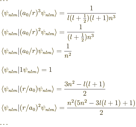 |
(D.60) |
where  is the Bohr radius, about 0.53 Å. Note that you can get
the expectation value of a more general function of by summing
terms, provided that the function can be expanded into a Laurent
series. Also note that the value of
is the Bohr radius, about 0.53 Å. Note that you can get
the expectation value of a more general function of by summing
terms, provided that the function can be expanded into a Laurent
series. Also note that the value of  does not make a difference:
you can combine of different values together and it
does not change the above expectation values. And watch it, when the
power of becomes too negative, the expectation value will cease to
exist. For example, for
does not make a difference:
you can combine of different values together and it
does not change the above expectation values. And watch it, when the
power of becomes too negative, the expectation value will cease to
exist. For example, for 
 0 the expectation values of
  and higher powers are infinite.
The trickiest to derive is the expectation value of  ,
and that one will be done first. First recall the hydrogen
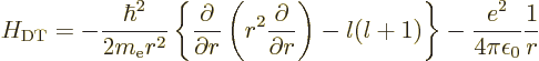
Hamiltonian from chapter 4.3,
,
and that one will be done first. First recall the hydrogen
Hamiltonian from chapter 4.3,
Its energy eigenfunctions of given square and  angular momentum
and their energy are
angular momentum
and their energy are
where the  are called the spherical harmonics.
When this Hamiltonian is applied to an eigenfunction
, it produces the exact same result as the following
dirty trick Hamiltonian
in which the angular
derivatives have been replaced by  :
:
The reason is that the angular derivatives are essentially the square
angular momentum operator of chapter 4.2.3. Now, while in
the hydrogen Hamiltonian the quantum number has to be an integer
because of its origin, in the dirty trick one can be allowed to
assume any value. That means that you can differentiate the
Hamiltonian and its eigenvalues  with respect to . And
that allows you to apply the Hellmann-Feynman theorem of section
A.38.1:
with respect to . And
that allows you to apply the Hellmann-Feynman theorem of section
A.38.1:
(Yes, the eigenfunctions are good, because the purely
radial  commutes with both
  and
and  , which
are angular derivatives.) Substituting in the dirty trick
Hamiltonian,
, which
are angular derivatives.) Substituting in the dirty trick
Hamiltonian,
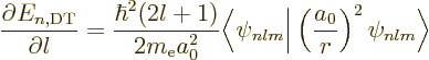
So, if you can figure out how the dirty trick energy changes with
near some desired integer value  , the desired
expectation value of at that integer value of follows.
Note that the eigenfunctions of can still be taken to be
of the form
, the desired
expectation value of at that integer value of follows.
Note that the eigenfunctions of can still be taken to be
of the form  , where
  can be divided out of the eigenvalue problem to give

 . If you skim back
through chapter 4.3 and its note, you see that that
eigenvalue problem was solved in derivation {D.15}.
Now, of course, is no longer an integer, but if you skim through
the note, it really makes almost no difference. The energy
eigenvalues are still
. If you skim back
through chapter 4.3 and its note, you see that that
eigenvalue problem was solved in derivation {D.15}.
Now, of course, is no longer an integer, but if you skim through
the note, it really makes almost no difference. The energy
eigenvalues are still 


 . If you look near the end of
the note, you see that the requirement on
. If you look near the end of
the note, you see that the requirement on  is that
 where
where  must remain an integer for valid solutions, hence
must stay constant under small changes. So
must remain an integer for valid solutions, hence
must stay constant under small changes. So 
 1, and then according to the chain rule the derivative of
 is
is  . Substitute it in
and there you have that nasty expectation value as given in
(D.60).
. Substitute it in
and there you have that nasty expectation value as given in
(D.60).
All other expectation values of  for integer values of
may be found from the “Kramers relation,” or “(second) Pasternack relation:”
for integer values of
may be found from the “Kramers relation,” or “(second) Pasternack relation:”
![\begin{displaymath}
4(q+1) \left\langle{q}\right\rangle
- 4 n^2(2q+1) \langle q-1\rangle
+ n^2 q[(2l+1)^2 - q^2] \langle q-2\rangle
= 0
\end{displaymath}](img7727.gif) |
(D.61) |
where  is shorthand for the expectation value
 .
.
Substituting 0 into the Kramers-Pasternack relation produces
the expectation value of as in (D.60). It may be
noted that this can instead be derived from the virial theorem of
chapter 7.2, or from the Hellmann-Feynman theorem by
differentiating the hydrogen Hamiltonian with respect to the charge
 . Substituting in 1, 2, ...produces the
expectation values for
. Substituting in 1, 2, ...produces the
expectation values for  ,
,  , ....
Substituting in 1 and the expectation value for
from the Hellmann-Feynman theorem gives the expectation
value for . The remaining negative integer values
2, 3, ...produce the remaining expectation values
for the negative integer powers of as the
, ....
Substituting in 1 and the expectation value for
from the Hellmann-Feynman theorem gives the expectation
value for . The remaining negative integer values
2, 3, ...produce the remaining expectation values
for the negative integer powers of as the
 term in the equation.
Note that for a sufficiently negative powers of , the
expectation value becomes infinite. Specifically, since
is proportional to  , {D.15}, it can be seen
that
, {D.15}, it can be seen
that  becomes infinite when
 . When that happens, the coefficient of the expectation
value in the Kramers-Pasternack relation becomes zero, making it
impossible to compute the expectation value. The relationship can be
used until it crashes and then the remaining expectation values are
all infinite.
. When that happens, the coefficient of the expectation
value in the Kramers-Pasternack relation becomes zero, making it
impossible to compute the expectation value. The relationship can be
used until it crashes and then the remaining expectation values are
all infinite.
The remainder of this note derives the Kramers-Pasternack relation.
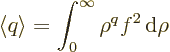
First note that the expectation values are defined as
When this integral is written in spherical coordinates, the
integration of the square spherical harmonic over the angular
coordinates produces one. So, the expectation value simplifies to
To simplify the notations, a nondimensional radial coordinate
 will be used. Also, a new radial function


 will be defined. In those terms,
the expression above for the expectation value shortens to
will be defined. In those terms,
the expression above for the expectation value shortens to
To further shorten the notations, from now on the limits of
integration and  will be omitted throughout. In those
notations, the expectation value of is
will be omitted throughout. In those
notations, the expectation value of is
Also note that the integrals are improper. It is to be assumed that
the integrations are from a very small value of to a very large
one, and that only at the end of the derivation, the limit is taken
that the integration limits become zero and infinity.
According to derivation {D.15}, the function  satisfies
in terms of the ordinary differential equation.
satisfies
in terms of the ordinary differential equation.
where primes indicate derivatives with respect to .
Substituting in  , you get
in terms of the new unknown function that
, you get
in terms of the new unknown function that
![\begin{displaymath}
f'' =
\left[
\frac{1}{n^2}-\frac{2}{\rho}+\frac{l(l+1)}{\rho^2}
\right]f %
\end{displaymath}](img7743.gif) |
(D.62) |
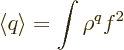
Since this makes  proportional to , forming the integral
 produces a combination of terms of the form
 , hence of expectation values of
powers of :
, hence of expectation values of
powers of :
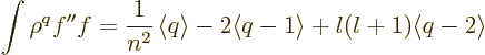 |
(D.63) |
The idea is now to apply integration by parts on to
produce a different combination of expectation values. The fact that
the two combinations must be equal will then give the
Kramers-Pasternack relation.
Before embarking on this, first note that since
the latter from integration by parts, it follows that
 |
(D.64) |
This result will be used routinely in the manipulations below to
reduce integrals of that form.
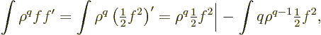
Now an obvious first integration by parts on produces
The first of the two integrals reduces to an expectation value of
 using (D.64). For the final integral, use
another integration by parts, but make sure you do not run around in a
circle because if you do you will get a trivial expression. What
works is integrating
using (D.64). For the final integral, use
another integration by parts, but make sure you do not run around in a
circle because if you do you will get a trivial expression. What
works is integrating  and differentiating
  :
:
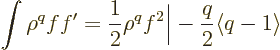
 |
(D.65) |
In the final integral, according to the differential equation
(D.62), the factor can be replaced by powers of
times :
and each of the terms is of the form (D.64), so you get
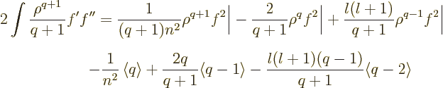
Plugging this into (D.65) and then equating that to
(D.63) produces the Kramers-Pasternack relation. It
also gives an additional right hand side
but that term becomes zero when the integration limits take their
final values zero and infinity. In particular, the upper limit values
always become zero in the limit of the upper bound going to infinity;
and its derivative go to zero exponentially then, beating out any
power of . The lower limit values also become zero in the
region of applicability that exists, because
that requires that  is for small proportional to
a power of greater than zero.
is for small proportional to
a power of greater than zero.
The above analysis is not valid when 1, since then the
final integration by parts would produce a logarithm, but since the
expression is valid for any other , not just integer ones you
can just take a limit  to cover that case.


![\begin{displaymath}
- \rho^2 R_{nl}'' - 2\rho R_{nl}'
+ \left[l(l+1)-2\rho+\frac{1}{n^2}\rho^2\right]R_{nl} = 0
\end{displaymath}](img7741.gif)

![\begin{displaymath}
2 \int\frac{\rho^{q+1}}{q+1}f'f'' =
2 \int\frac{\rho^{q+1}...
...t[\frac{1}{n^2}-\frac{2}{\rho}+\frac{l(l+1)}{\rho^2}\right]ff'
\end{displaymath}](img7755.gif)