4.3 The Hy­dro­gen Atom

This sec­tion ex­am­ines the crit­i­cally im­por­tant case of the hy­dro­gen atom. The hy­dro­gen atom con­sists of a nu­cleus which is just a sin­gle pro­ton, and an elec­tron en­cir­cling that nu­cleus. The nu­cleus, be­ing much heav­ier than the elec­tron, can be as­sumed to be at rest, and only the mo­tion of the elec­tron is of con­cern.

The en­ergy lev­els of the elec­tron de­ter­mine the pho­tons that the atom will ab­sorb or emit, al­low­ing the pow­er­ful sci­en­tific tool of spec­tral analy­sis. The elec­tronic struc­ture is also es­sen­tial for un­der­stand­ing the prop­er­ties of the other el­e­ments and of chem­i­cal bonds.

4.3.1 The Hamil­ton­ian

The first step is to find the Hamil­ton­ian of the elec­tron. The elec­tron ex­pe­ri­ences an elec­tro­sta­tic Coulomb at­trac­tion to the op­po­sitely charged nu­cleus. The cor­re­spond­ing po­ten­tial en­ergy is

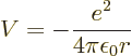$$V = -\frac{e^2}{4\pi\epsilon_0 r}$$ (4.28)

with $r$ the dis­tance from the nu­cleus. The con­stant

$$e \approx \mbox{1.602\,176\,6~10$\POW9,{-19}$\ C}$$ (4.29)

is the mag­ni­tude of the elec­tric charges of the elec­tron and pro­ton, and the con­stant

$$\epsilon_0 \approx \mbox{8.854\,187\,817~10$\POW9,{-12}$\ C$\POW9,{2}$/J m}$$ (4.30)

is called the “per­mit­tiv­ity of space.”

Un­like for the har­monic os­cil­la­tor dis­cussed ear­lier, this po­ten­tial en­ergy can­not be split into sep­a­rate parts for Carte­sian co­or­di­nates $x$, $y$, and $z$. To do the analy­sis for the hy­dro­gen atom, you must put the nu­cleus at the ori­gin of the co­or­di­nate sys­tem and use spher­i­cal co­or­di­nates $r$ (the dis­tance from the nu­cleus), $\theta$ (the an­gle from an ar­bi­trar­ily cho­sen $z$-​axis), and $\phi$ (the an­gle around the $z$-​axis); see fig­ure 4.7. In terms of spher­i­cal co­or­di­nates, the po­ten­tial en­ergy above de­pends on just the sin­gle co­or­di­nate $r$.

To get the Hamil­ton­ian, you need to add to this po­ten­tial en­ergy the ki­netic en­ergy op­er­a­tor ${\widehat T}$. Chap­ter 3.3 gave this op­er­a­tor as

$${\widehat T}= - \frac{\hbar^2}{2m} \nabla^2$$

where $\nabla^2$ is the Lapla­cian. The Lapla­cian in spher­i­cal co­or­di­nates is given in the no­ta­tions, (N.5). Then the Hamil­ton­ian is found to be:

$$H = - \frac{\hbar^2}{2m_{\rm e}r^2} \left\{ \frac{\parti... ...rtial \phi^2} \right\} - \frac{e^2}{4\pi\epsilon_0}\frac1r %$$ (4.31)

where

$$m_{\rm e}\approx \mbox{9.109~10$\POW9,{-31}$\ kg}$$ (4.32)

is the mass of the elec­tron.

It may be noted that the small pro­ton mo­tion can be cor­rected for by slightly ad­just­ing the mass of the elec­tron to be an ef­fec­tive 9.104 4 10$\POW9,{-31}$ kg, {A.5}. This makes the so­lu­tion ex­act, ex­cept for ex­tremely small er­rors due to rel­a­tivis­tic ef­fects. (These are dis­cussed in ad­den­dum {A.39}.)

Key Points

$\begin{picture}(15,5.5)(0,-3) \put(2,0){\makebox(0,0){\scriptsize\bf0}} \put(12... ...\thicklines \put(3,0){\line(1,0){12}}\put(11.5,-2){\line(1,0){3}} \end{picture}$

To an­a­lyze the hy­dro­gen atom, you must use spher­i­cal co­or­di­nates.

$\begin{picture}(15,5.5)(0,-3) \put(2,0){\makebox(0,0){\scriptsize\bf0}} \put(12... ...\thicklines \put(3,0){\line(1,0){12}}\put(11.5,-2){\line(1,0){3}} \end{picture}$

The Hamil­ton­ian in spher­i­cal co­or­di­nates has been writ­ten down. It is (4.31).

4.3.2 So­lu­tion us­ing sep­a­ra­tion of vari­ables

This sub­sec­tion de­scribes in gen­eral lines how the eigen­value prob­lem for the elec­tron of the hy­dro­gen atom is solved. The ba­sic ideas are like those used to solve the par­ti­cle in a pipe and the har­monic os­cil­la­tor, but in this case, they are used in spher­i­cal co­or­di­nates rather than Carte­sian ones. With­out get­ting too much caught up in the math­e­mat­i­cal de­tails, do not miss the op­por­tu­nity of learn­ing where the hy­dro­gen en­ergy eigen­func­tions and eigen­val­ues come from. This is the crown jewel of quan­tum me­chan­ics; bril­liant, al­most flaw­less, crit­i­cally im­por­tant; one of the great­est works of phys­i­cal analy­sis ever.

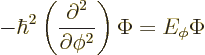
The eigen­value prob­lem for the Hamil­ton­ian, as for­mu­lated in the pre­vi­ous sub­sec­tion, can be solved by search­ing for so­lu­tions $\psi$ that take the form of a prod­uct of func­tions of each of the three co­or­di­nates: $\psi$ $\vphantom0\raisebox{1.5pt}{$=$}$ $R(r)\Theta(\theta)\Phi(\phi)$. More con­cisely, $\psi$ $\vphantom0\raisebox{1.5pt}{$=$}$ $R\Theta\Phi$. The prob­lem now is to find sep­a­rate equa­tions for the in­di­vid­ual func­tions $R$, $\Theta$, and $\Phi$ from which they can then be iden­ti­fied. The ar­gu­ments are sim­i­lar as for the har­monic os­cil­la­tor, but messier, since the co­or­di­nates are more en­tan­gled. First, sub­sti­tut­ing $\psi$ $\vphantom0\raisebox{1.5pt}{$=$}$ $R\Theta\Phi$ into the Hamil­ton­ian eigen­value prob­lem $H\psi$ $\vphantom0\raisebox{1.5pt}{$=$}$ $E\psi$, with the Hamil­ton­ian $H$ as given in the pre­vi­ous sub­sec­tion and $E$ the en­ergy eigen­value, pro­duces:

$$\begin{array}{r} \displaystyle \left[ - \frac{\hbar^2}{2... ...heta\Phi\; \\ [15pt] \displaystyle= E R\Theta\Phi \end{array}$$

To re­duce this prob­lem, pre­mul­ti­ply by $2{m_{\rm e}}r^2$$\raisebox{.5pt}{$/$}$​$R\Theta\Phi$ and then sep­a­rate the var­i­ous terms:

$$\begin{array}[b]{r} \displaystyle - \frac{\hbar^2}{R} \f... ... e^2}{4\pi\epsilon_0}\frac1r = 2m_{\rm e}r^2 E \end{array} %$$ (4.33)

Next iden­tify the terms in­volv­ing the an­gu­lar de­riv­a­tives and name them $E_{\theta\phi}$. They are:

$$\frac{1}{\Theta\Phi} \left[ -\frac{\hbar^2}{\sin\theta} ... ...ial^2}{\partial \phi^2} \right] \Theta\Phi = E_{\theta\phi}$$

By this de­f­i­n­i­tion, $E_{\theta\phi}$ only de­pends on $\theta$ and $\phi$, not $r$. But it can­not de­pend on $\theta$ or $\phi$ ei­ther, since none of the other terms in the orig­i­nal equa­tion (4.33) de­pends on them. So $E_{\theta\phi}$ must be a con­stant, in­de­pen­dent of all three co­or­di­nates. Then mul­ti­ply­ing the an­gu­lar terms above by $\Theta\Phi$ pro­duces a re­duced eigen­value prob­lem in­volv­ing $\Theta\Phi$ only, with eigen­value $E_{\theta\phi}$:

$$\left[ -\frac{\hbar^2}{\sin\theta} \frac{\partial}{\parti... ...al \phi^2} \right] \Theta\Phi = E_{\theta\phi} \Theta\Phi %$$ (4.34)

Re­peat the game with this re­duced eigen­value prob­lem. Mul­ti­ply by $\sin^2\theta$$\raisebox{.5pt}{$/$}$​$\Theta\Phi$, and name the only $\phi$-​de­pen­dent term $E_\phi$. It is:

$$- \frac{1}{\Phi} \hbar^2 \left( \frac{\partial^2}{\partial\phi^2} \right) \Phi = E_\phi$$

By de­f­i­n­i­tion $E_\phi$ only de­pends on $\phi$, but since the other two terms in the equa­tion it came from did not de­pend on $\phi$, $E_\phi$ can­not ei­ther, so it must be an­other con­stant. What is left is a sim­ple eigen­value prob­lem just in­volv­ing $\Phi$:

$$- \hbar^2 \left( \frac{\partial^2}{\partial\phi^2} \right) \Phi = E_\phi \Phi$$

And that is read­ily solv­able.

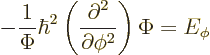
In fact, the so­lu­tion to this fi­nal prob­lem has al­ready been given, since the op­er­a­tor in­volved is just the square of the an­gu­lar mo­men­tum op­er­a­tor $\L _z$ of sec­tion 4.2.2:

$$- \hbar^2 \left( \frac{\partial^2}{\partial\phi^2} \righ... ...frac{\partial}{\partial\phi} \right)^2 \Phi = \L _z^2 \Phi$$

So this equa­tion must have the same eigen­func­tions as the op­er­a­tor $\L _z$,

$$\Phi_m=e^{{\rm i}m\phi}$$

and must have the square eigen­val­ues

$$E_\phi=(m\hbar)^2$$

(each ap­pli­ca­tion of $\L _z$ mul­ti­plies the eigen­func­tion by $m\hbar$). It may be re­called that the mag­netic quan­tum num­ber $m$ must be an in­te­ger.

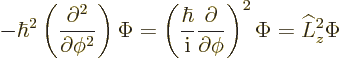
The eigen­value prob­lem (4.34) for $\Theta\Phi$ is even eas­ier; it is ex­actly the one for the square an­gu­lar mo­men­tum $L^2$ of sec­tion 4.2.3. (So, no, there was not re­ally a need to solve for $\Phi$ sep­a­rately.) Its eigen­func­tions are there­fore the spher­i­cal har­mon­ics,

$$\Theta\Phi = Y_l^m(\theta,\phi)$$

and its eigen­val­ues are

$$E_{\theta\phi} = l (l+1) \hbar^2$$

It may be re­called that the az­imuthal quan­tum num­ber $l$ must be an in­te­ger greater than or equal to $\vert m\vert$.

Re­turn­ing now to the so­lu­tion of the orig­i­nal eigen­value prob­lem (4.33), re­place­ment of the an­gu­lar terms by $E_{\theta\phi}$ $\vphantom0\raisebox{1.5pt}{$=$}$ $l(l+1)\hbar^2$ turns it into an or­di­nary dif­fer­en­tial equa­tion prob­lem for the ra­dial fac­tor $R(r)$ in the en­ergy eigen­func­tion. As usual, this prob­lem is a pain to solve, so that is again shoved away in a note, {D.15}.

It turns out that the so­lu­tions of the ra­dial prob­lem can be num­bered us­ing a third quan­tum num­ber, $n$, called the “prin­ci­pal quan­tum num­ber”. It is larger than the az­imuthal quan­tum num­ber $l$, which in turn must be at least as large as the ab­solute value of the mag­netic quan­tum num­ber:

$$\fbox{$\displaystyle n > l \mathrel{\raisebox{-1pt}{$\geqslant$}}\vert m\vert $}$$ (4.35)

so the prin­ci­pal quan­tum num­ber must be at least 1. And if $n$ $\vphantom0\raisebox{1.5pt}{$=$}$ 1, then $l$ $\vphantom0\raisebox{1.5pt}{$=$}$ $m$ $\vphantom0\raisebox{1.5pt}{$=$}$ 0.

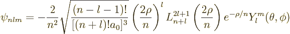
In terms of these three quan­tum num­bers, the fi­nal en­ergy eigen­func­tions of the hy­dro­gen atom are of the gen­eral form:

$$\fbox{$\displaystyle \psi_{nlm} = R_{nl}(r) Y_l^m(\theta,\phi) $} %$$ (4.36)

where the spher­i­cal har­mon­ics $Y_l^m$ were de­scribed in sec­tion 4.2.3. The brand new ra­dial wave func­tions $R_{nl}$ can be found writ­ten out in ta­ble 4.4 for small val­ues of $n$ and $l$, or in de­riva­tion {D.15}, (D.8), for any $n$ and $l$. 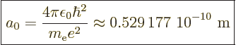They are usu­ally writ­ten in terms of a scaled ra­dial dis­tance from the nu­cleus $\rho$ $\vphantom0\raisebox{1.5pt}{$=$}$ $r$$\raisebox{.5pt}{$/$}$​$a_0$, where the length $a_0$ is called the Bohr ra­dius and has the value

$$\fbox{$\displaystyle a_0=\frac{4\pi\epsilon_0\hbar^2}{m_{\rm e}e^2} \approx \mbox{0.529\,177~10$\POW9,{-10}$\ m} $} %$$ (4.37)

or about half an Ångstrom. The Bohr ra­dius is a re­ally good length scale to de­scribe atoms in terms of. The Ångstrom it­self is a good choice too, it is 10$\POW9,{-10}$ m, or one tenth of a nanome­ter.

Ta­ble 4.4: The first few ra­dial wave func­tions for hy­dro­gen.

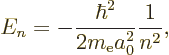
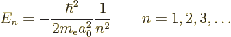
The en­ergy eigen­val­ues are much sim­pler and more in­ter­est­ing than the eigen­func­tions; they are

$$\fbox{$\displaystyle E_n = - \frac{\hbar^2}{2 m_{\rm e}a_... ...\frac{\hbar^2}{2 m_{\rm e}a_0^2} = - \mbox{13.605\,7 eV} $} %$$ (4.38)

where eV stands for elec­tron volt, a unit of en­ergy equal to 1.602 18 10$\POW9,{-19}$ J. It is the en­ergy that an elec­tron picks up dur­ing a 1 volt change in elec­tric po­ten­tial.

You may won­der why the en­ergy only de­pends on the prin­ci­pal quan­tum num­ber $n$, and not also on the az­imuthal quan­tum num­ber $l$ and the mag­netic quan­tum num­ber $m$. Well, the choice of $z$-​axis was ar­bi­trary, so it should not seem that strange that the physics would not de­pend on the an­gu­lar mo­men­tum in that di­rec­tion. But that the en­ergy does not de­pend on $l$ is non­triv­ial: if you solve the sim­pler prob­lem of a par­ti­cle stuck in­side an im­pen­e­tra­ble spher­i­cal con­tainer, us­ing pro­ce­dures from {A.6}, the en­ergy val­ues de­pend on both $n$ and $l$. So, that is just the way it is. (It stops be­ing true any­way if you in­clude rel­a­tivis­tic ef­fects in the Hamil­ton­ian.)

Since the low­est pos­si­ble value of the prin­ci­pal quan­tum num­ber $n$ is one, the ground state of low­est en­ergy $E_1$ is eigen­func­tion $\psi_{100}$.

Key Points

$\begin{picture}(15,5.5)(0,-3) \put(2,0){\makebox(0,0){\scriptsize\bf0}} \put(12... ...\thicklines \put(3,0){\line(1,0){12}}\put(11.5,-2){\line(1,0){3}} \end{picture}$

Skip­ping a lot of math, en­ergy eigen­func­tions $\psi_{nlm}$ and their en­ergy eigen­val­ues $E_n$ have been found.

$\begin{picture}(15,5.5)(0,-3) \put(2,0){\makebox(0,0){\scriptsize\bf0}} \put(12... ...\thicklines \put(3,0){\line(1,0){12}}\put(11.5,-2){\line(1,0){3}} \end{picture}$

There is one eigen­func­tion for each set of three in­te­ger quan­tum num­bers $n$, $l$, and $m$ sat­is­fy­ing $n$ $\raisebox{.3pt}{$>$}$ $l$ $\raisebox{-.5pt}{$\geqslant$}$ $\vert m\vert$. The num­ber $n$ is called the prin­ci­pal quan­tum num­ber.

$\begin{picture}(15,5.5)(0,-3) \put(2,0){\makebox(0,0){\scriptsize\bf0}} \put(12... ...\thicklines \put(3,0){\line(1,0){12}}\put(11.5,-2){\line(1,0){3}} \end{picture}$

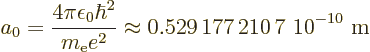
The typ­i­cal length scale in the so­lu­tion is called the Bohr ra­dius $a_0$, which is about half an Ångstrom.

$\begin{picture}(15,5.5)(0,-3) \put(2,0){\makebox(0,0){\scriptsize\bf0}} \put(12... ...\thicklines \put(3,0){\line(1,0){12}}\put(11.5,-2){\line(1,0){3}} \end{picture}$

The de­rived eigen­func­tions $\psi_{nlm}$ are eigen­func­tions of

• $z$ an­gu­lar mo­men­tum, with eigen­value $L_z$ $\vphantom0\raisebox{1.5pt}{$=$}$ $m\hbar$;
• square an­gu­lar mo­men­tum, with eigen­value $L^2$ $\vphantom0\raisebox{1.5pt}{$=$}$ $l(l+1)\hbar^2$;
• en­ergy, with eigen­value $E_n$ $\vphantom0\raisebox{1.5pt}{$=$}$ $\vphantom{0}\raisebox{1.5pt}{$-$}$$\hbar^2$$\raisebox{.5pt}{$/$}$​$2{m_{\rm e}}a_0^2n^2$.

$\begin{picture}(15,5.5)(0,-3) \put(2,0){\makebox(0,0){\scriptsize\bf0}} \put(12... ...\thicklines \put(3,0){\line(1,0){12}}\put(11.5,-2){\line(1,0){3}} \end{picture}$

The en­ergy val­ues only de­pend on the prin­ci­pal quan­tum num­ber $n$.

$\begin{picture}(15,5.5)(0,-3) \put(2,0){\makebox(0,0){\scriptsize\bf0}} \put(12... ...\thicklines \put(3,0){\line(1,0){12}}\put(11.5,-2){\line(1,0){3}} \end{picture}$

The ground state is $\psi_{100}$.

4.3.2 Re­view Ques­tions

1.

Use the ta­bles for the ra­dial wave func­tions and the spher­i­cal har­mon­ics to write down the wave func­tion

$$\psi_{nlm} = R_{nl}(r) Y_l^m(\theta ,\phi)$$

for the case of the ground state $\psi_{100}$.

Check that the state is nor­mal­ized. Note: $\int_0^{\infty}e^{-2u}u^2{\,\rm d}{u}$ $\vphantom0\raisebox{1.5pt}{$=$}$ $\frac 14$.

So­lu­tion hydb-a

2.

Use the generic ex­pres­sion

$$\psi_{nlm} = -\frac{2}{n^2} \sqrt{\frac{(n-l-1)!}{[(n+l)!a_0... ...+1}\left(\frac{2\rho}n\right) e^{-\rho /n} Y_l^m(\theta ,\phi)$$

with $\rho$ $\vphantom0\raisebox{1.5pt}{$=$}$ $r$$\raisebox{.5pt}{$/$}$​$a_0$ and $Y_l^m$ from the spher­i­cal har­mon­ics ta­ble to find the ground state wave func­tion $\psi_{100}$. Note: the La­guerre poly­no­mial $L_1(x)$ $\vphantom0\raisebox{1.5pt}{$=$}$ $1-x$ and for any $p$, $L_1^p$ is just its $p$-​th de­riv­a­tive.

So­lu­tion hydb-b

3.

Plug num­bers into the generic ex­pres­sion for the en­ergy eigen­val­ues,

$$E_n = - \frac{\hbar^2}{2m_{\rm e}a_0^2} \frac 1{n^2},$$

where $a_0$ $\vphantom0\raisebox{1.5pt}{$=$}$ $4\pi\epsilon_0\hbar^2$$\raisebox{.5pt}{$/$}$​${m_{\rm e}}e^2$, to find the ground state en­ergy. Ex­press in eV, where 1 eV equals 1.602 2 10$\POW9,{-19}$ J. Val­ues for the phys­i­cal con­stants can be found at the start of this sec­tion and in the no­ta­tions sec­tion.

So­lu­tion hydb-c

4.3.3 Dis­cus­sion of the eigen­val­ues

The only en­ergy val­ues that the elec­tron in the hy­dro­gen atom can have are the “Bohr en­er­gies” de­rived in the pre­vi­ous sub­sec­tion:

$$E_n = - \frac{\hbar^2}{2 m_{\rm e}a_0^2} \frac1{n^2} \qquad n = 1, 2, 3, \ldots$$

This sub­sec­tion dis­cusses the phys­i­cal con­se­quences of this re­sult.

Fig­ure 4.8: Spec­trum of the hy­dro­gen atom.

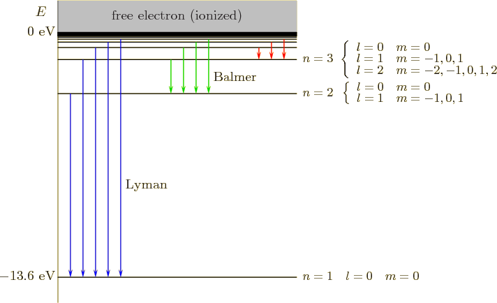
To aid the dis­cus­sion, the al­lowed en­er­gies are plot­ted in the form of an en­ergy spec­trum in fig­ure 4.8. To the right of the low­est three en­ergy lev­els the val­ues of the quan­tum num­bers that give rise to those en­ergy lev­els are listed.

The first thing that the en­ergy spec­trum il­lus­trates is that the en­ergy lev­els are all neg­a­tive, un­like the ones of the har­monic os­cil­la­tor, which were all pos­i­tive. How­ever, that does not mean much; it re­sults from defin­ing the po­ten­tial en­ergy of the har­monic os­cil­la­tor to be zero at the nom­i­nal po­si­tion of the par­ti­cle, while the hy­dro­gen po­ten­tial is in­stead de­fined to be zero at large dis­tance from the nu­cleus. (It will be shown later, chap­ter 7.2, that the av­er­age po­ten­tial en­ergy is twice the value of the to­tal en­ergy, and the av­er­age ki­netic en­ergy is mi­nus the to­tal en­ergy, mak­ing the av­er­age ki­netic en­ergy pos­i­tive as it should be.)

A more pro­found dif­fer­ence is that the en­ergy lev­els of the hy­dro­gen atom have a max­i­mum value, namely zero, while those of the har­monic os­cil­la­tor went all the way to in­fin­ity. It means phys­i­cally that while the par­ti­cle can never es­cape in a har­monic os­cil­la­tor, in a hy­dro­gen atom, the elec­tron es­capes if its to­tal en­ergy is greater than zero. Such a loss of the elec­tron is called “ion­iza­tion” of the atom.

There is again a ground state of low­est en­ergy; it has to­tal en­ergy

$$E_1=-13.6 \mbox{ eV} %$$ (4.39)

(an eV or elec­tron volt is 1.6 10$\POW9,{-19}$ J). The ground state is the state in which the hy­dro­gen atom will be at ab­solute zero tem­per­a­ture. In fact, it will still be in the ground state at room tem­per­a­ture, since even then the en­ergy of heat mo­tion is un­likely to raise the en­ergy level of the elec­tron to the next higher one, $E_2$.

The ion­iza­tion en­ergy of the hy­dro­gen atom is 13.6 eV; this is the min­i­mum amount of en­ergy that must be added to raise the elec­tron from the ground state to the state of a free elec­tron.

If the elec­tron is ex­cited from the ground state to a higher but still bound en­ergy level, (maybe by pass­ing a spark through hy­dro­gen gas), it will in time again tran­si­tion back to a lower en­ergy level. Dis­cus­sion of the rea­sons and the time evo­lu­tion of this process will have to wait un­til chap­ter 7. For now, it can be pointed out that dif­fer­ent tran­si­tions are pos­si­ble, as in­di­cated by the ar­rows in fig­ure 4.8. They are named by their fi­nal en­ergy level to be Ly­man, Balmer, or Paschen se­ries tran­si­tions.

The en­ergy lost by the elec­tron dur­ing a tran­si­tion is emit­ted as a quan­tum of elec­tro­mag­netic ra­di­a­tion called a pho­ton. The most en­er­getic pho­tons, in the ul­tra­vi­o­let range, are emit­ted by Ly­man tran­si­tions. Balmer tran­si­tions emit vis­i­ble light and Paschen ones in­frared.

The pho­tons emit­ted by iso­lated atoms at rest must have an en­ergy very pre­cisely equal to the dif­fer­ence in en­ergy eigen­val­ues; any­thing else would vi­o­late the re­quire­ment of the or­tho­dox in­ter­pre­ta­tion that only the eigen­val­ues are ob­serv­able. And ac­cord­ing to the “Planck-Ein­stein re­la­tion,” the pho­ton’s en­ergy equals the an­gu­lar fre­quency $\omega$ of its elec­tro­mag­netic vi­bra­tion times $\hbar$:

$$E_{n_1}-E_{n_2} = \hbar \omega.$$

Thus the spec­trum of the light emit­ted by hy­dro­gen atoms is very dis­tinc­tive and can be iden­ti­fied to great ac­cu­racy. Dif­fer­ent el­e­ments have dif­fer­ent spec­tra, and so do mol­e­cules. It all al­lows atoms and mol­e­cules to be cor­rectly rec­og­nized in a lab or out in space.

(To be sure, the spec­tral fre­quen­cies are not truly math­e­mat­i­cally ex­act num­bers. A slight spec­tral broad­en­ing is un­avoid­able be­cause no atom is truly iso­lated as as­sumed here; there is al­ways some ra­di­a­tion that per­turbs it even in the most ideal empty space. In ad­di­tion, ther­mal mo­tion of the atom causes Doppler shifts. In short, only the en­ergy eigen­val­ues are ob­serv­able, but ex­actly what those eigen­val­ues are for a real-life atom can vary slightly.)

Atoms and mol­e­cules may also ab­sorb elec­tro­mag­netic en­ergy of the same fre­quen­cies that they can emit. That al­lows them to en­ter an ex­cited state. The ex­cited state will even­tu­ally emit the ab­sorbed en­ergy again in a dif­fer­ent di­rec­tion, and pos­si­bly at dif­fer­ent fre­quen­cies by us­ing dif­fer­ent tran­si­tions. In this way, in as­tron­omy atoms can re­move spe­cific fre­quen­cies from light that passes them on its way to earth, re­sult­ing in an ab­sorp­tion spec­trum. Or in­stead atoms may scat­ter spe­cific fre­quen­cies of light in our di­rec­tion that was orig­i­nally not headed to earth, pro­duc­ing an emis­sion spec­trum. Doppler shifts can pro­vide in­for­ma­tion about the ther­mal and av­er­age mo­tion of the atoms. Since hy­dro­gen is so preva­lent in the uni­verse, its en­ergy lev­els as de­rived here are par­tic­u­larly im­por­tant in as­tron­omy. Chap­ter 7 will ad­dress the mech­a­nisms of emis­sion and ab­sorp­tion in much greater de­tail.

Key Points

$\begin{picture}(15,5.5)(0,-3) \put(2,0){\makebox(0,0){\scriptsize\bf0}} \put(12... ...\thicklines \put(3,0){\line(1,0){12}}\put(11.5,-2){\line(1,0){3}} \end{picture}$

The en­ergy lev­els of the elec­tron in a hy­dro­gen atom have a high­est value. This en­ergy is by con­ven­tion taken to be the zero level.

$\begin{picture}(15,5.5)(0,-3) \put(2,0){\makebox(0,0){\scriptsize\bf0}} \put(12... ...\thicklines \put(3,0){\line(1,0){12}}\put(11.5,-2){\line(1,0){3}} \end{picture}$

The ground state has a en­ergy 13.6 eV be­low this zero level.

$\begin{picture}(15,5.5)(0,-3) \put(2,0){\makebox(0,0){\scriptsize\bf0}} \put(12... ...\thicklines \put(3,0){\line(1,0){12}}\put(11.5,-2){\line(1,0){3}} \end{picture}$

If the elec­tron in the ground state is given an ad­di­tional amount of en­ergy that ex­ceeds the 13.6 eV, it has enough en­ergy to es­cape from the nu­cleus. This is called ion­iza­tion of the atom.

$\begin{picture}(15,5.5)(0,-3) \put(2,0){\makebox(0,0){\scriptsize\bf0}} \put(12... ...\thicklines \put(3,0){\line(1,0){12}}\put(11.5,-2){\line(1,0){3}} \end{picture}$

If the elec­tron tran­si­tions from a bound en­ergy state with a higher prin­ci­pal quan­tum num­ber $n_1$ to a lower one $n_2$, it emits ra­di­a­tion with an an­gu­lar fre­quency $\omega$ given by

$$\hbar \omega = E_{n_1}-E_{n_2}$$

$\begin{picture}(15,5.5)(0,-3) \put(2,0){\makebox(0,0){\scriptsize\bf0}} \put(12... ...\thicklines \put(3,0){\line(1,0){12}}\put(11.5,-2){\line(1,0){3}} \end{picture}$

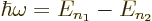
Sim­i­larly, atoms with en­ergy $E_{n_2}$ may ab­sorb elec­tro­mag­netic en­ergy of such a fre­quency.

4.3.3 Re­view Ques­tions

1.

If there are in­fi­nitely many en­ergy lev­els $E_1$, $E_2$, $E_3$, $E_4$, $E_5$, $E_6$, ..., where did they all go in the en­ergy spec­trum?

So­lu­tion hydc-a

2.

What is the value of en­ergy level $E_2$? And $E_3$?

So­lu­tion hydc-b

3.

Based on the re­sults of the pre­vi­ous ques­tion, what is the color of the light emit­ted in a Balmer tran­si­tion from en­ergy $E_3$ to $E_2$? The Planck-Ein­stein re­la­tion says that the an­gu­lar fre­quency $\omega$ of the emit­ted pho­ton is its en­ergy di­vided by $\hbar$, and the wave length of light is $2{\pi}c$$\raisebox{.5pt}{$/$}$​$\omega$ where $c$ is the speed of light. Typ­i­cal wave lengths of vis­i­ble light are: vi­o­let 400 nm, in­digo 445 nm, blue 475 nm, green 510 nm, yel­low 570 nm, or­ange 590 nm, red 650 nm.

So­lu­tion hydc-c

4.

What is the color of the light emit­ted in a Balmer tran­si­tion from an en­ergy level $E_n$ with a high value of $n$ to $E_2$?

So­lu­tion hydc-d

4.3.4 Dis­cus­sion of the eigen­func­tions

The ap­pear­ance of the en­ergy eigen­states will be of great in­ter­est in un­der­stand­ing the heav­ier el­e­ments and chem­i­cal bonds. This sub­sec­tion de­scribes the most im­por­tant of them.

It may be re­called from sub­sec­tion 4.3.2 that there is one eigen­func­tion $\psi_{nlm}$ for each set of three in­te­ger quan­tum num­bers. They are the prin­ci­pal quan­tum num­ber $n$ (de­ter­min­ing the en­ergy of the state), the az­imuthal quan­tum num­ber $l$ (de­ter­min­ing the square an­gu­lar mo­men­tum), and the mag­netic quan­tum num­ber $m$ (de­ter­min­ing the an­gu­lar mo­men­tum in the cho­sen $z$-​di­rec­tion.) They must sat­isfy the re­quire­ments that

$$n > l \mathrel{\raisebox{-1pt}{$\geqslant$}}\vert m\vert$$

For the ground state, with the low­est en­ergy $E_1$, $n$ $\vphantom0\raisebox{1.5pt}{$=$}$ 1 and hence ac­cord­ing to the con­di­tions above both $l$ and $m$ must be zero. So the ground state eigen­func­tion is $\psi_{100}$; it is unique.

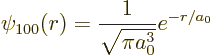
The ex­pres­sion for the wave func­tion of the ground state is (from the re­sults of sub­sec­tion 4.3.2):

$$\psi_{100}(r) = \frac{1}{\sqrt{\pi a_0^3}} e^{-r/a_0} %$$ (4.40)

where $a_0$ is called the “Bohr ra­dius”,

$$a_0 = \frac{4\pi\epsilon_0\hbar^2}{m_{\rm e}e^2} \approx \mbox{0.529\,177\,210\,7~10$\POW9,{-10}$\ m}$$ (4.41)

The square mag­ni­tude of the en­ergy states will again be dis­played as grey tones, darker re­gions cor­re­spond­ing to re­gions where the elec­tron is more likely to be found. The ground state is shown this way in fig­ure 4.9; the elec­tron may be found within a blob size that is about three times the Bohr ra­dius, or roughly an Ångstrom, (10$\POW9,{-10}$ m), in di­am­e­ter.

Fig­ure 4.9: Ground state wave func­tion of the hy­dro­gen atom.

It is the quan­tum me­chan­i­cal re­fusal of elec­trons to re­strict them­selves to a sin­gle lo­ca­tion that gives atoms their size. If Planck's con­stant $\hbar$ would have been zero, so would have been the Bohr ra­dius, and the elec­tron would have been in the nu­cleus. It would have been a very dif­fer­ent world.

The ground state prob­a­bil­ity dis­tri­b­u­tion is spher­i­cally sym­met­ric: the prob­a­bil­ity of find­ing the elec­tron at a point de­pends on the dis­tance from the nu­cleus, but not on the an­gu­lar ori­en­ta­tion rel­a­tive to it.

The ex­cited en­ergy lev­els $E_2$, $E_3$, ...are all de­gen­er­ate; as the spec­trum fig­ure 4.8 in­di­cated, there is more than one eigen­state pro­duc­ing each level. Let’s have a look at the states at en­ergy level $E_2$ now.

Fig­ure 4.10 shows en­ergy eigen­func­tion $\psi_{200}$. Like $\psi_{100}$, it is spher­i­cally sym­met­ric. In fact, all eigen­func­tions $\psi_{n00}$ are spher­i­cally sym­met­ric. How­ever, the wave func­tion has blown up a lot, and now sep­a­rates into a small, more or less spher­i­cal re­gion in the cen­ter, sur­rounded by a sec­ond re­gion that forms a spher­i­cal shell. Sep­a­rat­ing the two is a ra­dius at which there is zero prob­a­bil­ity of find­ing the elec­tron.

Fig­ure 4.10: Eigen­func­tion $\psi_{200}$.

The state $\psi_{200}$ is com­monly re­ferred to as the 2s state. The 2 in­di­cates that it is a state with en­ergy $E_2$. The “s” in­di­cates that the az­imuthal quan­tum num­ber is zero; just think spher­i­cally sym­met­ric. Sim­i­larly, the ground state $\psi_{100}$ is com­monly in­di­cated as 1s, hav­ing the low­est en­ergy $E_1$.

States which have az­imuthal quan­tum num­ber $l$ $\vphantom0\raisebox{1.5pt}{$=$}$ 1 are called “p” states, for some his­tor­i­cal rea­son. His­tor­i­cally, physi­cists have al­ways loved con­fus­ing and in­con­sis­tent no­ta­tions. In par­tic­u­lar, the $\psi_{21m}$ states are called 2p states. As first ex­am­ple of such a state, fig­ure 4.11 shows $\psi_{210}$. This wave func­tion squeezes it­self close to the $z$-​axis, which is plot­ted hor­i­zon­tally by con­ven­tion. There is zero prob­a­bil­ity of find­ing the elec­tron at the ver­ti­cal $x,y$ sym­me­try plane, and max­i­mum prob­a­bil­ity at two sym­met­ric points on the $z$-​axis.

Fig­ure 4.11: Eigen­func­tion $\psi_{210}$, or 2p$_z$.

Since the wave func­tion squeezes close to the $z$-​axis, this state is of­ten more specif­i­cally re­ferred to as the 2p$_z$ state. Think “points along the $z$-​axis.”

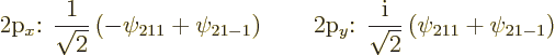
Fig­ure 4.12 shows the other two 2p states, $\psi_{211}$ and $\psi_{21-1}$. These two states look ex­actly the same as far as the prob­a­bil­ity den­sity is con­cerned. It is some­what hard to see in the fig­ure, but they re­ally take the shape of a torus around the left-to-right $z$-​axis.

Fig­ure 4.12: Eigen­func­tion $\psi_{211}$ (and $\psi_{21-1}$).

Eigen­func­tions $\psi_{200}$, $\psi_{210}$, $\psi_{211}$, and $\psi_{21-1}$ are de­gen­er­ate: they all four have the same en­ergy $E_2$ $\vphantom0\raisebox{1.5pt}{$=$}$ $\vphantom{0}\raisebox{1.5pt}{$-$}$3.4 eV. The con­se­quence is that they are not unique. Com­bi­na­tions of them can be formed that have the same en­ergy. These com­bi­na­tion states may be more im­por­tant phys­i­cally than the orig­i­nal eigen­func­tions.

In par­tic­u­lar, the torus-shaped eigen­func­tions $\psi_{211}$ and $\psi_{21-1}$ are of­ten not very use­ful for de­scrip­tions of heav­ier el­e­ments and chem­i­cal bonds. Two states that are more likely to be rel­e­vant here are called 2p$_x$ and 2p$_y$; they are the com­bi­na­tion states:

$$\mbox{2p$_x$: } \frac1{\sqrt2}\left(-\psi_{211}+\psi_{21-1}... ...$: } \frac{{\rm i}}{\sqrt2}\left(\psi_{211}+\psi_{21-1}\right)$$ (4.42)

These two states are shown in fig­ure 4.13; they look ex­actly like the pointer state 2p$_z$ of fig­ure 4.11, ex­cept that they squeeze along the $x$-​axis, re­spec­tively the $y$-​axis, in­stead of along the $z$-​axis. (Since the $y$-​axis is point­ing to­wards you, 2p$_y$ looks ro­ta­tion­ally sym­met­ric. Seen from the side, it would look like p$_z$ in fig­ure 4.11.)

Fig­ure 4.13: Eigen­func­tions 2p$_x$, left, and 2p$_y$, right.

Note that un­like the two orig­i­nal states $\psi_{211}$ and $\psi_{21-1}$, the states 2p$_x$ and 2p$_y$ do not have a def­i­nite value of the $z$-​com­po­nent of an­gu­lar mo­men­tum; the $z$-​com­po­nent has a 50/50 un­cer­tainty of be­ing ei­ther $+\hbar$ or $\vphantom{0}\raisebox{1.5pt}{$-$}$$\hbar$. But that is not im­por­tant in most cir­cum­stances. What is im­por­tant is that when mul­ti­ple elec­trons oc­cupy the p states, mu­tual re­pul­sion ef­fects tend to push them into the p$_x$, p$_y$, and p$_z$ states.

So, the four in­de­pen­dent eigen­func­tions at en­ergy level $E_2$ are best thought of as con­sist­ing of one spher­i­cally sym­met­ri­cal 2s state, and three di­rec­tional states, 2p$_x$, 2p$_y$, and 2p$_z$, point­ing along the three co­or­di­nate axes.

But even that is not al­ways ideal; as dis­cussed in chap­ter 5.11.4, for many chem­i­cal bonds, es­pe­cially those in­volv­ing the im­por­tant el­e­ment car­bon, still dif­fer­ent com­bi­na­tion states called hy­brids show up. They in­volve com­bi­na­tions of the 2s and the 2p states and there­fore have un­cer­tain square an­gu­lar mo­men­tum as well.

Key Points

$\begin{picture}(15,5.5)(0,-3) \put(2,0){\makebox(0,0){\scriptsize\bf0}} \put(12... ...\thicklines \put(3,0){\line(1,0){12}}\put(11.5,-2){\line(1,0){3}} \end{picture}$

The typ­i­cal size of eigen­states is given by the Bohr ra­dius, mak­ing the size of the atom of the or­der of an Å.

$\begin{picture}(15,5.5)(0,-3) \put(2,0){\makebox(0,0){\scriptsize\bf0}} \put(12... ...\thicklines \put(3,0){\line(1,0){12}}\put(11.5,-2){\line(1,0){3}} \end{picture}$

The ground state $\psi_{100}$, or 1s state, is non­de­gen­er­ate: no other set of quan­tum num­bers $n,l,m$ pro­duces en­ergy $E_1$.

$\begin{picture}(15,5.5)(0,-3) \put(2,0){\makebox(0,0){\scriptsize\bf0}} \put(12... ...\thicklines \put(3,0){\line(1,0){12}}\put(11.5,-2){\line(1,0){3}} \end{picture}$

All higher en­ergy lev­els are de­gen­er­ate, there is more than one eigen­state pro­duc­ing that en­ergy.

$\begin{picture}(15,5.5)(0,-3) \put(2,0){\makebox(0,0){\scriptsize\bf0}} \put(12... ...\thicklines \put(3,0){\line(1,0){12}}\put(11.5,-2){\line(1,0){3}} \end{picture}$

All states of the form $\psi_{n00}$, in­clud­ing the ground state, are spher­i­cally sym­met­ric, and are called s states. The ground state $\psi_{100}$ is the 1s state, $\psi_{200}$ is the 2s state, etcetera.

$\begin{picture}(15,5.5)(0,-3) \put(2,0){\makebox(0,0){\scriptsize\bf0}} \put(12... ...\thicklines \put(3,0){\line(1,0){12}}\put(11.5,-2){\line(1,0){3}} \end{picture}$

States of the form $\psi_{n1m}$ are called p states. The ba­sic 2p states are $\psi_{21-1}$, $\psi_{210}$, and $\psi_{211}$.

$\begin{picture}(15,5.5)(0,-3) \put(2,0){\makebox(0,0){\scriptsize\bf0}} \put(12... ...\thicklines \put(3,0){\line(1,0){12}}\put(11.5,-2){\line(1,0){3}} \end{picture}$

The state $\psi_{210}$ is also called the 2p$_z$ state, since it squeezes it­self around the $z$-​axis.

$\begin{picture}(15,5.5)(0,-3) \put(2,0){\makebox(0,0){\scriptsize\bf0}} \put(12... ...\thicklines \put(3,0){\line(1,0){12}}\put(11.5,-2){\line(1,0){3}} \end{picture}$

There are sim­i­lar 2p$_x$ and 2p$_y$ states that squeeze around the $x$ and $y$ axes. Each is a com­bi­na­tion of $\psi_{21-1}$ and $\psi_{211}$.

$\begin{picture}(15,5.5)(0,-3) \put(2,0){\makebox(0,0){\scriptsize\bf0}} \put(12... ...\thicklines \put(3,0){\line(1,0){12}}\put(11.5,-2){\line(1,0){3}} \end{picture}$

The four spa­tial states at the $E_2$ en­ergy level can there­fore be thought of as one spher­i­cally sym­met­ric 2s state and three 2p pointer states along the axes.

$\begin{picture}(15,5.5)(0,-3) \put(2,0){\makebox(0,0){\scriptsize\bf0}} \put(12... ...\thicklines \put(3,0){\line(1,0){12}}\put(11.5,-2){\line(1,0){3}} \end{picture}$

How­ever, since the $E_2$ en­ergy level is de­gen­er­ate, eigen­states of still dif­fer­ent shapes are likely to show up in ap­pli­ca­tions.

4.3.4 Re­view Ques­tions

1.

At what dis­tance $r$ from the nu­cleus does the square of the ground state wave func­tion be­come less than one per­cent of its value at the nu­cleus? Ex­press it both as a mul­ti­ple of the Bohr ra­dius $a_0$ and in Å.

So­lu­tion hydd-a

2.

Check from the con­di­tions

$$n > l \mathrel{\raisebox{-1pt}{$\geqslant$}}\vert m\vert$$

that $\psi_{200}$, $\psi_{211}$, $\psi_{210}$, and $\psi_{21-1}$ are the only states of the form $\psi_{nlm}$ that have en­ergy $E_2$. (Of course, all their com­bi­na­tions, like 2p$_x$ and 2p$_y$, have en­ergy $E_2$ too, but they are not sim­ply of the form $\psi_{nlm}$, but com­bi­na­tions of the ba­sic so­lu­tions $\psi_{200}$, $\psi_{211}$, $\psi_{210}$, and $\psi_{21-1}$.)

So­lu­tion hydd-b

3.

Check that the states

$$\mbox{2p$_x$}= \frac 1{\sqrt 2}\left(-\psi_{211}+\psi_{21-1}... ...$}= \frac{{\rm i}}{\sqrt 2}\left(\psi_{211}+\psi_{21-1}\right)$$

are prop­erly nor­mal­ized.

So­lu­tion hydd-c